Abstract

The purpose of the study was to tie economics and physics together by the analysis of maximizing utility functions through the use of LaGrange multipliers. This study was made of a computationally simulated economy made of 100 agents with unique preferences that make trades out of the 5 possible goods within the system, all acting with the intention of maximizing their own unique utility function. The simulation is tested for basic economic theories such as supply, demand, and inflation. Multiple simulations were run in testing for theoretically expected money utility derived by the use of Lagrange Multipliers. The results were that the theorized expectation of money utility as being acceptable in that the agents had near constant levels of money utility with respect to all goods. The simulation was also tested under separate initial conditions of money supply, goods available, and preferences to show results of basic economic theories of supply, demand, and inflation were present through the reactionary measurement of the prices of goods as the initial conditions were altered.

Introductory Material

Introduction:

Introduction: Physics and Economics hold similarities such that they both describe the surrounding world. With that, analogies can be made from one field to the other. Because of this Econophysics as a field has caught on as of recent. Econophysics was first noticed within the mid 1990’s by Physicists that were working in the field of statistical mechanics. It has since gained traction through the years with more development in areas that tie Physics and Economics together. The purpose of the new field is to be able to better describe financial systems with the use of Physics. Over the years analogies from Physics have been drawn to Economics and Finance, laws such as the inverse power law which is heavily used in Physics being used to relate returns and volatility of equities, Omori processes relating major volatilities in markets to that of mini-shockwaves which occur after large earthquakes (Weber), and thermodynamic relationships with variables in equity markets. The fields of economics, and physics continuing to merge together show that there are alternative ways to look at financial markets. The financial world now has increasingly larger amounts of data available, ranging from minute pricing data of stocks, to macroscopic economic data regarding nations. The availability of the data allows for the field of finance to depend on a quantitative outlook, making use of mathematics and physics. This allows the possibility for testing of theories which were once only limited to stay within their initial fields. Utility theories relation to both classical mechanics and thermodynamics is the most well-known discoveries which relate economics with physics. For years utility was known and used to make sense of how individuals behaved. There is the basic belief that each and every individual makes decisions with the purpose of maximizing their own utility. The theory from economics can be described with Physics through the use of thermodynamics relating utility to entropy and classical mechanics use of maximizing utility functions (Smith and Foley). It is common for the field of economics to use Lagrange multipliers for optimizations such as, utility, resources, labor etc... The purpose of this project is to showcase that there is an analogy between Physics and Economics through the use of Lagrange Multipliers. The project will be a simulation of an economy which consists of agents, goods and money. The economy will allow for trade between agents that act based on maximizing their individual utility. Utility in this simulation is the driving force behind in which why these agents chose to buy and sell their goods, it can be thought of as synonymous to happiness or satisfaction. The Utility function will depend on goods and each agent will be trying to maximize their utility based on their individual preferences for each good. The total utility function will be equal to the sum of utility gained from individual goods. There is a total of 5 goods within the economy and the preferences for each good will be hardcoded and allowed for the simulation to gather data. Ideally the agents should be smart enough to trade with one another in where both parties of the trade go in the direction of maximizing their individual utilities. The prices for goods will depend on how much each agent is willing to ask or bid for the good. Previous transaction prices will be stored because the asking and biding of goods will be based on historical transactions. Agents will all start with equal initial amounts of money and goods. The simulation will run with hardcoded given initial conditions of goods, money, and preferences. Tweaking of these initial conditions will be used for each simulation to show analogy between Physics and Economics. The iterations for the simulations were chosen depending on scenario. Ultimately as iterations get large enough the agents’ overall utility will maximize and plateau, meaning they get to a point in which trading amongst each other stops. This is the point where equilibrium is rea. When the system arrives at equilibrium, relationships between the economic simulation and thermodynamics can be made. Overall, the simulation will consist of agents that are all trying to maximize their utility eventually arriving at equilibrium. Once equilibrium is reached the system will be described using thermodynamic relations and be available for the use of Lagrange multipliers.

Background:

Utility:

Utility theory shows a framework in the description of why individuals make certain decisions. It is used as a measure of how much satisfaction an individual gains by the choices they make, and units of measurement are referred to as utils. Individuals can be seen to have utility functions based on their preferences, income, and prices of goods available. Utility functions can be used to describe behaviors and choices that individuals make. The simulation created will consist of agents that will interact with one another through the trading of goods, in order to maximize their own unique utility functions. Their utility functions are dependent on the goods available within the system, and all agents have hard-coded preferences and utility functions that depend on goods they possess. The simulation ran through thousands of iterations till the point in which all of the agents came to a noticeable equilibrium in terms of utility with respect to time.

Preferences:

Preferences can be seen as analogous to demand. Agents within the simulation have a hardcoded utility function which depends on the amount of goods they possess. Each good holds a unique value of utility depending on the agent. The utility value gained by the individual good depends on the preference set for each agent. The preference differentiates the amount of utility that each good holds for each agent. This becomes a factor when agents are deciding on trades to make that maximize their utility by the largest amount of utils. The graph below shows an example of two different agents utility function for the same good.

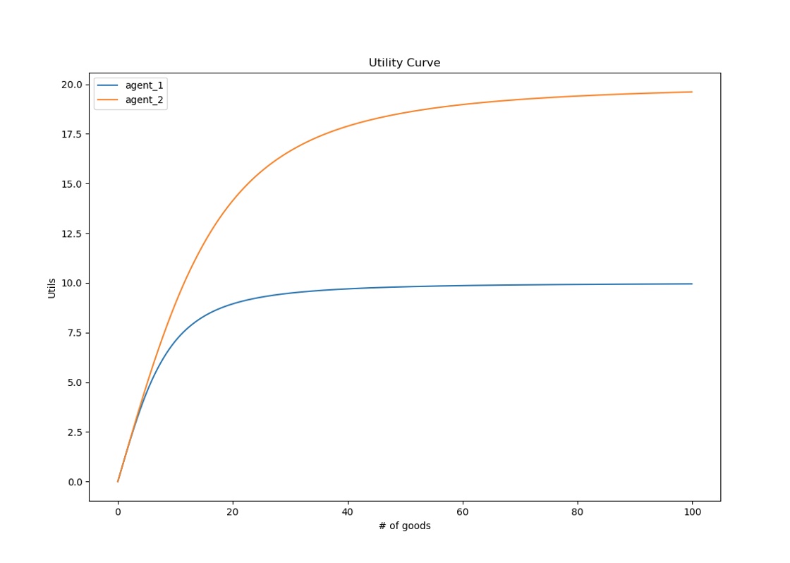
The graph demonstrates the differences in utility for each agent regarding the same good. Agent 1’s curve shows that more of the good is required for him to get to a point in which the gain in utils for each good start to diminish. In comparison agent 2 see’s this diminishing return of utility for the good at a much earlier stage of goods obtained. These curves are dependent on the preference held by each agent for the considered good. It shows that agent 1 has a larger preference for the good than agent 2, because the return on utility for each additional good does not reach its plateau until a larger amount of that good is obtained. The total utility curve for each agent is the summation of utility curves for each good, and all agents use their utility curves in maximizing their total utility when making trades.

Supply and Demand:

Supply and demand curves deal with the relationships between the quantity of goods demanded and the prices at which these goods are sold. Supply deals with the manufacturers side with the quantity of goods which the suppliers are willing to produce. Suppliers have the incentive to increase supply in order to increase the prices which generates more profit, as long as it meets the demand for that good. The demand curve is how much consumers are willing to buy the product. It is a negatively sloped curve which decreases the price of the good as the quantity demanded increases. The sweet spot in which both curves intersect is known as the equilibrium price, and this represents the price at which the market maximizes the amount of goods supplied with the goods demanded. Manufacturers aim to be at the equilibrium price, any lower would be missing out on potential profit, and anything above would make for excess amount of goods produced.

inflation

Inflation is the rise in prices of goods or services that are impacted by variables such as demand-pull, cost-push, built-in, and monetaristic policy (Investopedia). The rise in prices of goods and services may be caused by high demand of the good, high costs associated with production of the good, and also the money supply effected by monetary policy. This simulation deals with the monetary policy aspect of demonstrating that inflation is existent. The system is closed, and the money supply is fixed throughout, meaning that no creation or destruction of money occurs through all iterations. What is tested is how the money supply affects the pricing of each good.

Theoretical Calculations and Lagrange Multipliers:

Lagrange multipliers is a mathematical method used to find maxima or minima of functions with given constraint equations representing the system. The project uses Lagrange Multipliers to show a derivation which ends up with a description of money utility for each agent within the system. When the system arrives at an equilibrium state, we make the assumptions that there is no change in price for all goods. This can imply that the net worth of an agent should be fixed as well, because it is a sum of both their liquid (cash) and hard assets (value of goods). This gives a constraint equation as shown below, and allows for the setting up of the Lagrange equation as shown below. With the Lagrange equation setup, the derivative is taken with respect to each good, which maximizes the utility for each agent and shows what the Lagrangian Multiplier ends up being.

The derivation above arrives at a conclusion in which the multiplier represents money utility in the economic system. The discovery of the Lagrangian multiplier states that once in equilibrium that the money utility for each agent should be constant for all goods. Theoretically this is what was tested for through the analysis of the data outputted by the simulation.

Expectations at Equilibrium

As the simulation is ran through it arrives at a state of equilibrium in terms of Utility per agent. This measurement is taken visually by the graphing of each agents utility function coming to a near constant level. When equilibrium is achieved the agents would ideally have no incentive to trade anymore because their utility has already been maximized to its full potential. When this occurs, the assumption is that trading no longer occurs and that the prices of goods should be constant along with the agents change in utility. Below is what is expected at equilibrium with respect to time for the simulation.

Methods Used

Overall the simulation when ran through enough iterations arrived at a noticeable equilibrium state. Being at an equilibrium state means that the agents all have maximized their utility through the trading of the goods that they prefer. Initially the system as a whole was not in equilibrium in that all of the agents were making trades that attempted to maximize their individual utilities. The system consisted of 5 different goods and the simulation ran with 100 total agents, all with unique preferences for goods. These preferences were hard coded and could be altered to test for demand, supply, inflation etc.… To start off the agents had fixed initial conditions such as money and the number of goods each agent possesses, these conditions were altered throughout separate simulations for specific testing. Any simulation that was tested required the system to arrive at an equilibrium state in terms of the agent’s utility becoming maximized. The figure below shows a simulation of 10,000 iterations in which all 100 agents arrived at a noticeable equilibrium state.

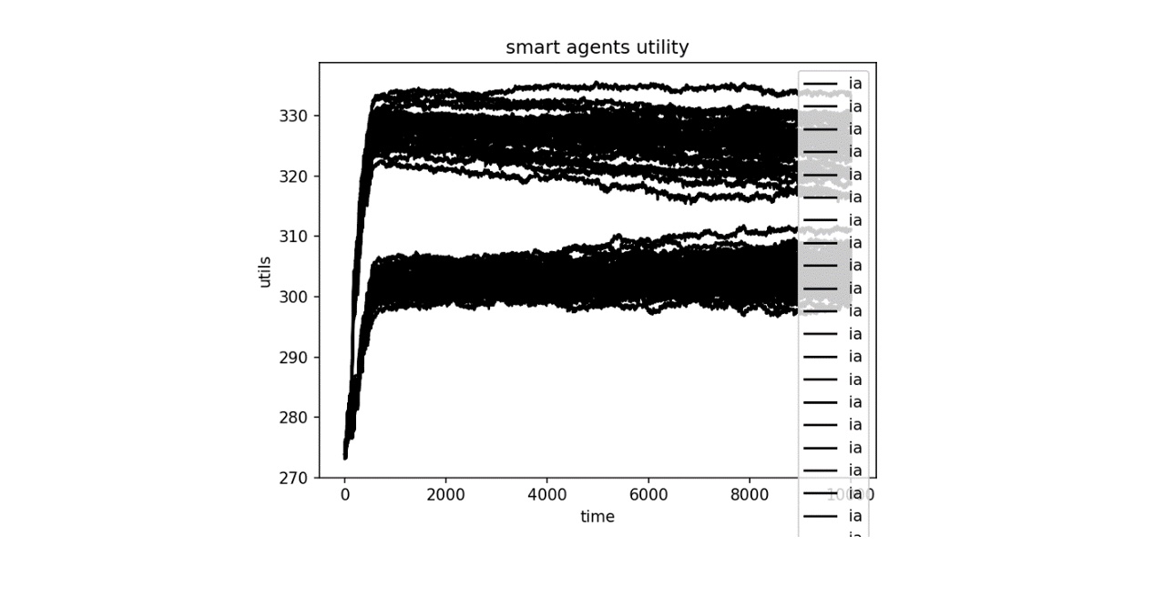
The graph above shows a simulation in which there are two different kinds of agents that eventually were seen to come to an equilibrium state. The state of equilibrium is when all the agents don’t have the need to trade because they have had the correct amount of goods that they possess. This is because they have made enough trades that have already maximized their individual utility. The system is not perfect, so the agent’s utility tends to oscillate minimally, but for the purpose of the project the assumption is that they have arrived at an equilibrium state. The analogies to thermodynamics can be compared only once the system is in supposed equilibrium. It is then that a look at certain variables such as the changes in price, goods, and utility with respect to time (iterations). Ideally each agent would come to a constant utility where no trading occurs, but experimentally the agents are not smart enough for an ideal equilibrium state to occur within the simulation. This is why it is noticeable that once the agents reach a certain utility there are small amounts of fluctuation in their utility graphs rather than arriving to a constant level. This is the point in which variables such as goods, prices, utility can all be measured to find analogies between the simulated system, and thermodynamics. Testing was done through multiple simulations with different initial conditions of money supply and goods available set to show that that the simulated system demonstrates fundamental economic theories such as supply and demand, inflation, and the theoretically expected results of money utility described by Lagrange Multipliers.

Results

Trial 1: Testing for Demand

The simulation showcases Demand theory of economics through the measurement of average prices of preferred goods with relation to the number of agents that have a strong preference for that good. For this project the preferences relate to the demand of that good. There are two kinds of agents A and B that have symmetric preferences for goods available. Agent A prefers good 0 the most while good1, 2,3, and 4 give Agent A the have lower amounts of utility gained respectively. Agent B has the opposite preference in that good 4 maximizes his utility while goods 3,2,1, and 0 have very lower impact on his utility respectively. Since all agents make decisions in trade with the motivation to maximize their utility, the preferences of goods can be seen as being analogous to the demand for goods. With that known, testing for demand of the simulation can be done by comparing the prices at which transactions are occurring against the percentage of Agents either A or B who make up the entire system. Below is the graph of multiple simulations graphed along with the percentage of Agent A’s that make up the whole system changing.

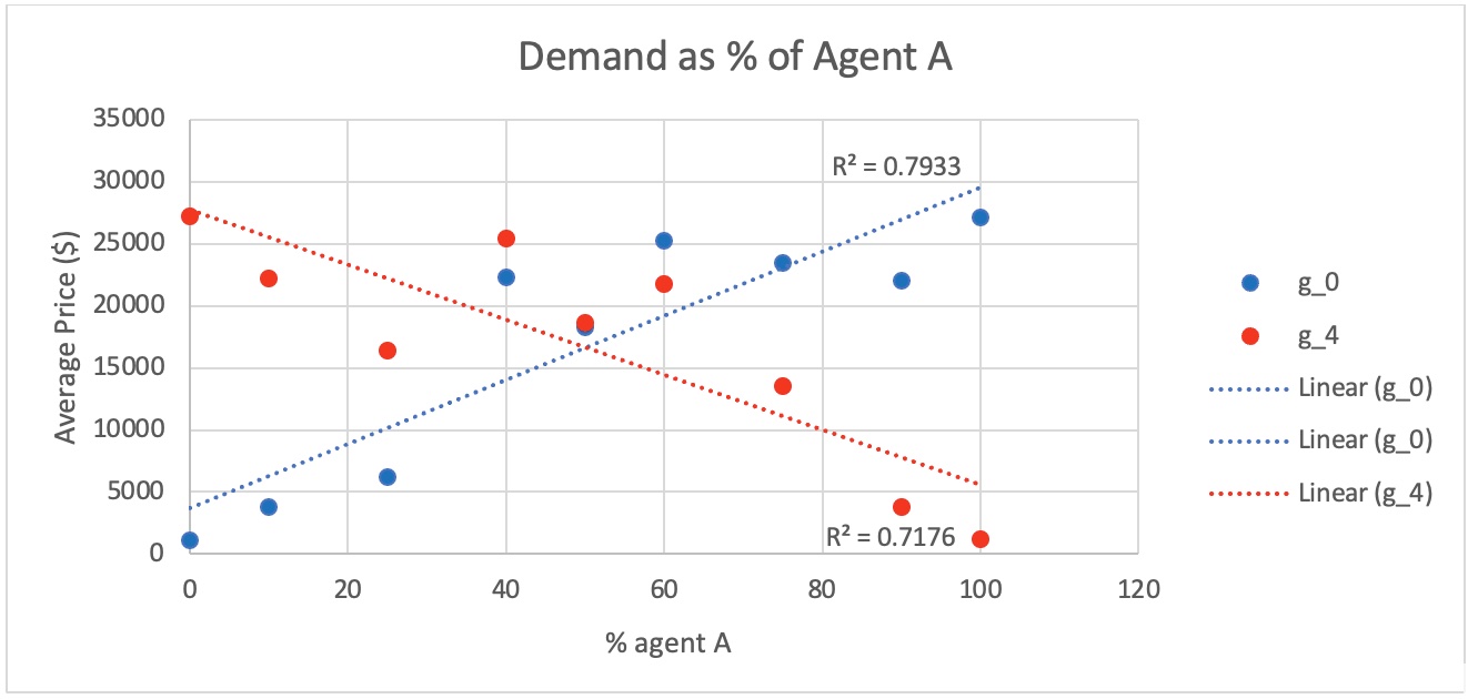
The graph above shows that demand is evident within the simulation through the average transaction price of the most preferred good relating to the demand by the agents who preferred it most. Good 0 increase as the % of Agent A’s making up the system increase, while the opposite affect shows the price of good 4 decreasing as the % of Agent B’s making up the system decreases. Number of simulations ran were 9 which the data was acquired, and the regression fit was able to achieve an r-squared value of .7933 for good 0 and 0.7176 for good 4. Results were not perfect, but still do an adequate job in showing the existence of demand within the simulation.

Trial 2: Testing for Supply

The economic theory of Supply was tested through gathering data over multiple simulations. Both Agents A’s and B’s start off with an initial supply of goods that they possess with money available being constant for all agents through all simulations. Once the simulation began, trades are made through each round where each agent makes transactions that reflect in maximizing their individual utility. Through this process, preferences for Agents A and B remain the same and symmetric as done so in trial 1 of Demand. Theoretically if the initial conditions of supply of goods each agent starts off with changes it should be reflected in the average price the goods were traded at. This would give an expected Supply curve in which the price goes down as the quantity of goods available increases. Testing this through 6 simulations that ran for 10,000 iterations each with increasing amounts of initial supply of all goods within the system results in the graph below.

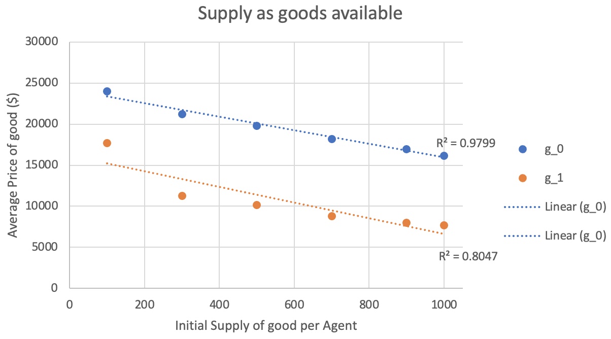
The graph above shows the decrease in average price of good 0 and 1 as the initial supply increases from 100 to 1000 units. It portrays an acceptable supply curve with r-squared values of good 0 being 0.9799 and good 1 being 0.8047. The downward sloping linear graph demonstrates that supply is evident within the simulation. Again, the conditions for this data is based on the simulation reaching a noticeable equilibrium state in which changes in prices, goods, and utility are all minimal. The reaching of an equilibrium state allows for the true value of pricing for all goods to be discovered.

Trial 3 Proof of Inflation:

This trial tests for the effects of inflation within the simulation. Inflation is thought of as how prices react accordingly to money supply. If an economy were to be injected with a large dosage of money, prices of goods should see an increase because variables such as costs, wages, and demand pushes prices up through the increase in money supply . In the simulations case, inflation was tested through the comparison of initial amounts of money that each agent starts off with to the average prices the goods reach once the system is in equilibrium. Inflation deals with money circulating within the economy, in this case the simulation is made up of the agents making trades. Taking into consideration the amount of money all agents have within their bank accounts, expectations are for inflation to be noticeable through the increase in average prices of the goods as the money supply (initial amount of money) increases. Below is a graph gathered from separate simulations with money supply changing from $100 to $2,000.

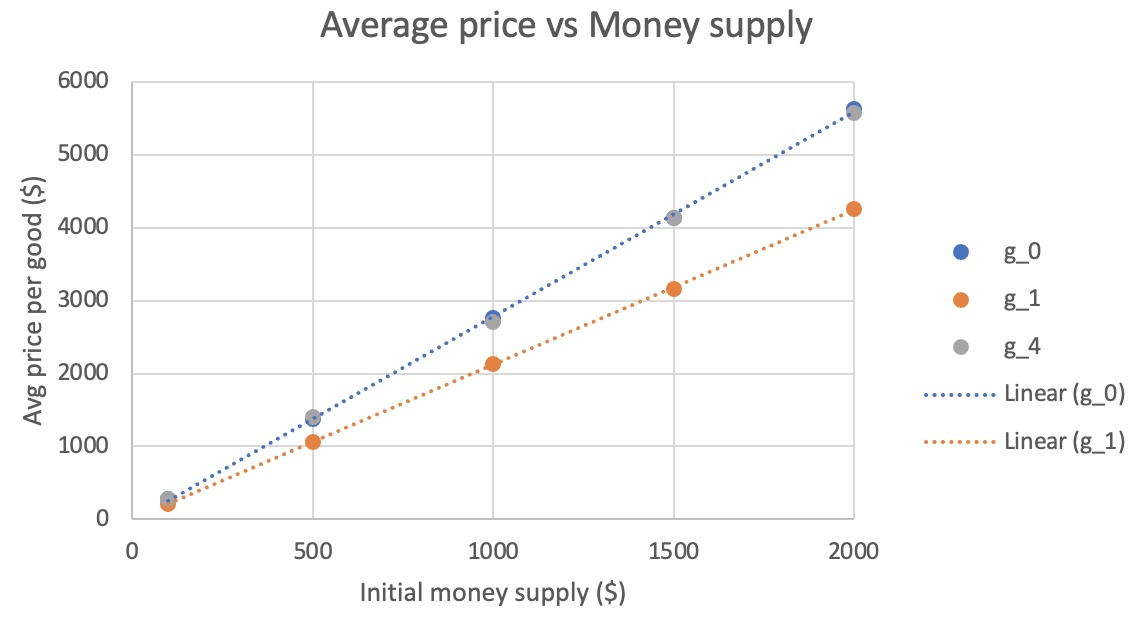
The graph above shows a linear relationship in which inflation follows. As there is an increase in the initial amounts of money which the agents start off with, the prices of the goods show an increase in a linear trend. Though the money supply does not mean pure circulation in the scenarios, it is affected by the increase in the agents asks/bids which is related to the funds they have available. There is a clear linear trend of inflation within the simulation which shows that the simulation behaves accordingly to basic economics.

Trial 4: Money Utility

When the system arrives at an equilibrium, the expectation is for trading to be minimal. This allows for the assumption that the agents have very little incentive for trading any further. Conclusion is that the money utility for each agent across all goods should be constant because trading is not preferred due to the state of equilibrium. Money utility is the amount of utils each dollar gives the agent. When the system arrives at an equilibrium each agent should have a constant money utility for all goods, derived from solving the Lagrangian multiplier in the Background section. Results for the constant level of money utility for agents are shown below.

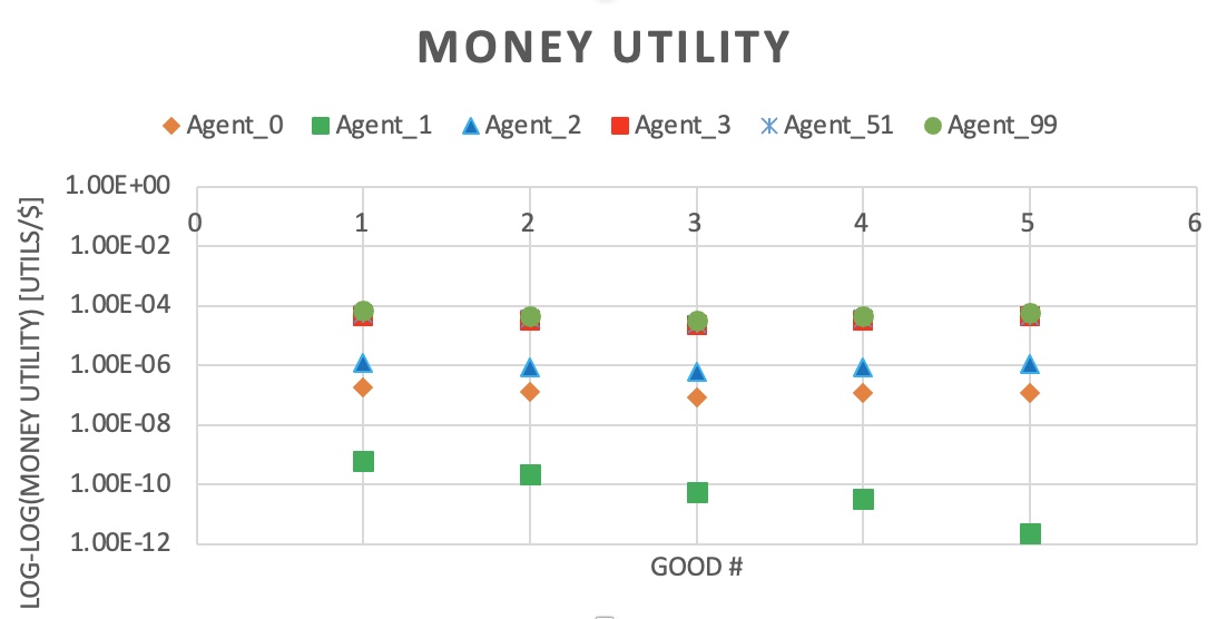
The graph above shows the money utility associated for four different agents. It is in log-log format for better visualization because of the agents having different orders of magnitude of money utility. Overall, the results look like it lines up with the expected theory of each agent having a near constant money utility across all goods. The reason for the differing in agents magnitude of money utility is because each agent started off with differing initial conditions of money and goods. Differences in initial conditions were given to differentiate the agents ability to arrive at equilibrium, which causes differences in both marginal and money utility for each agent. The simulation relating to the data above had gone through 5,000 iterations and had three types of agents (A,B,C) with different preferences. They type of agent did not affect the magnitude of money utility where as the differing conditions did. Agents 3, 51, 99 were different types of agents with differing preferences, and the graph above shows the three agents being overlapped. The reason for this is that these agents had a similar path to equilibrium which caused for similar values for the goods. Agents 0,1, and 2’s money utilities differ in magnitude from the other agents due to their unique initial conditions of money, and goods they started off with. The unique initial conditions caused for the agents to arrive at equilibrium in a different manner causing different values in which they viewed each good, affecting the magnitude of money utility. The data above shows that it falls in line with the hypothesis of each agent having a constant money utility across all goods once in an equilibrium state.

Conclusion

The objective of the simulation was to show that it describes fundamental economic market conditions of supply, demand, inflation, and to show that Lagrange Multipliers in a closed system could be used to describe the money utility. The results showed that supply, demand and inflation were all existent within the simulation. The theory of supply was tested for by increasing the amount of goods available and measuring the average price of the goods through multiple trials. This resulted in a decrease in average prices of goods in a linear fashion as expected of an economy which follows supply theory. Demand was showcased through changing the percentage of types of agents that the system contained. Two types of Agents (A and B) were a part of the system, both having different preferences for goods available. Multiple trials were run measuring the average transaction prices of the goods as the percent of Agent A’s and B’s within the system varied. The results showed an increase in the prices of the goods preferred most by the type of Agents making up the system, holding true to demand theory. Inflation was shown by the measurement of the average prices of goods increasing linearly as the amount of money supply increased. Overall, the simulation held true to fundamental economic theories of supply, demand, and inflation. The money utility portion of the system in equilibrium was expected to be near constant across all goods for each agent. Tested were three types of Agents (A, B, and C) that made up the total 100 agent system. Results showed that measured money utility across all goods for each type of Agent was near constant, confirming the initial hypothesis. Overall, the simulation gave evidence that it met practical market conditions and accurately tested the hypothesis of money utility in an equilibrium state of being constant across all goods for each agent.

References

Weber, P., Wang, F., Vodenska-Chitkushev, I., Havlin, S., & Stanley, H. E. (2007). Relation between volatility correlations in financial markets and Omori processes occurring on all scales. Physical Review E, 76(1), 016109.

Smith, E., & Foley, D. K. (2002). Is utility theory so different from thermodynamics?. SFI Working Paper 02-04-016.

Intriligator, M. D. (1971). Mathematical optimization and economic theory (Vol. 39). Siam.

Seth, S. (2018, October 31). Inflation Definition. Retrieved from https://www.investopedia.com/terms/i/inflation.asp

Code