Summary
This chapter focuses on volatility, mean and standard deviation, lognormal distributions, and the difference between realized and implied volatility. Volatility measures the speed of the market. Markets that move slow have low volatility, while markets that move fast have high volatility. Mean and standard deviation are looked at when observing a normal distribution. A nice example of a normal distribution demonstrated by the random walk of a pinbll going down a triangular maze of pegs and coming to a stop at bottom bins. Across each row the pinball touches a peg and has a 50/50 option of going either left or right. This is done as the pinball touches each peg for all the rows untill it reaches the bottom. If a large amount of pinballs through many iterations were to go down this maze there comes to what looks like a normal distribution with the mean at the center (right below where the pinball was originally dropped). Either going left or right from the center the count of pinballs in each bin get lesser making for tails on both the left and right edges. The random walk causes for a normal distribution, which intuitively makes sense. 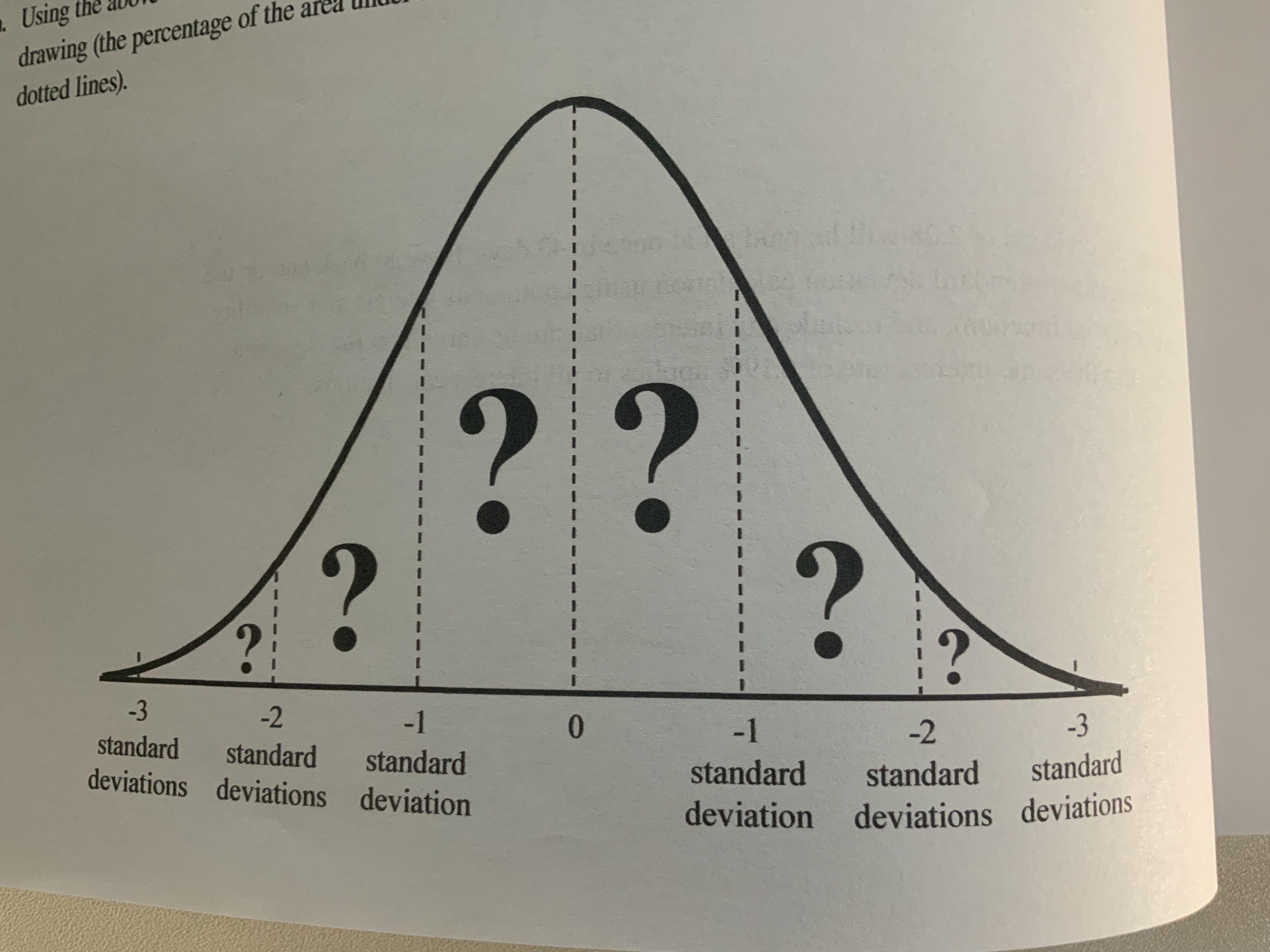You would expect the most amount of pinballs to collect at the center bin right underneath where the pinball was dropped, while the edges to be the least as it would mean that anytime the pinball encounters a peg it would go either left or right 100 % of the time to reach the edges. The mean is generally the peak of the distribution, while the standard deviation is how fast the distribution spreads out. The standard deviation tells us the likelihood of the ball ending up in a specific bin, and the probability of the ball ending up in a range of bins from the mean. Often known as sigma [-3,-2,-1,1,2,3] and the associated probabilities (68.3%, 95.4%, 99.7%). When looking at Options, volatility is synonymous to standard deviation. When we consider pricing of a stock it is known that it does not make a normal distribution. It's a lognormal distribution because there is a cap on the downside as stocks can't go below $0 and theoretically it can go to infinity on the upside. This makes the distribution non-symetrical and more in line with a lognormal distribution, showing a slight skew to the right side as the right tail possibilities are a bit fatter. Finally we come to the difference between realized and implied volatility. Realized volatility is calculated using the historical motion of the stock over a defined timeframe. Implied volatility is back calculated because it is a forecast of what the market believes will happen. To get a certain price of an Options contract 4 out of the 5 parameters are known, with implied volatility being left out. Knowing this implied volatility can be back calculated which shows us what the market is forecasting for that given stock.

Exercise problems:
1. t is a time period expressed in years, σ is the annual volatility and F is the forward futures price, then for simple volatility calculations (rather than exponential calculations) a price change of n standard deviations over the time period t can be approximated as: $$ n\times F \times \sigma \times \sqrt{t} $$ For a daily standard deviation, traders customarily assume 256 trading days in a year. $$ \textrm{t is therefore 1/256}, \textrm{and} \sqrt{t} = 1/16 $$ For a weekly standard deviation, assuming 52 trading weeks in a year, t is 1/52 and √t = 1/7.2
Using simple volatility calculations, and assuming that the forward price is equal to the current price, what is an approximate daily and weekly one standard deviation price change for each of the contracts below?
a. contract price = 78.00
Answer: \[ \begin{array}{|c|c|c|c|c|} \hline \text{Volatility} & \text{20%} & \text{30%} & \text{40%} & \text{50%} \\ \hline \text{daily standard deviation} & \pm0.98 & \pm1.46 & \pm1.95 & \pm2.44 \\ \hline \text{weekly standard deviation} & \pm2.16 & \pm3.24 & \pm4.33 &\pm5.41 \\ \hline \end{array} \] $$ n = 1, F = 78.00, \sigma = 0.20 $$ $$ \textrm{Daily = } 1 \times 78 \times 0.20 \times \sqrt{1/256} = \pm 0.98 $$ $$ \textrm{Weekly = } 1 \times 78 \times 0.20 \times \sqrt{1/52} = \pm 2.16 $$ b. contract price = 1,325.00
Answer: \[ \begin{array}{|c|c|c|c|c|} \hline \text{Volatility} & \text{10%} & \text{15%} & \text{20%} & \text{25%} \\ \hline \text{daily standard deviation} & \pm 8.28 & \pm 12.42 & \pm 16.56 & \pm 20.70 \\ \hline \text{weekly standard deviation} & \pm 18.37 & \pm 27.56 & \pm 36.75 &\pm 45.94 \\ \hline \end{array} \] c. contract price = 1.6270
Answer: \[ \begin{array}{|c|c|c|c|c|} \hline \text{Volatility} & \text{8%} & \text{10%} & \text{12%} & \text{14%} \\ \hline \text{daily standard deviation} & \pm 0.008 & \pm 0.010 & \pm 0.012 & \pm 0.014 \\ \hline \text{weekly standard deviation} & \pm 0.018 & \pm 0.023 & \pm 0.027 &\pm 0.032 \\ \hline \end{array} \] d. contract price = 669.00
Answer: \[ \begin{array}{|c|c|c|c|c|} \hline \text{Volatility} & \text{15%} & \text{23%} & \text{31%} & \text{39%} \\ \hline \text{daily standard deviation} & \pm 6.27 & \pm 9.62 & \pm 12.96 & \pm 16.31 \\ \hline \text{weekly standard deviation} & \pm 13.92 & \pm 21.34 & \pm 28.76 &\pm 36.18 \\ \hline \end{array} \] e. contract price = 3,187.00
Answer: \[ \begin{array}{|c|c|c|c|c|} \hline \text{Volatility} & \text{13%} & \text{17%} & \text{21%} & \text{25%} \\ \hline \text{daily standard deviation} & \pm 25.89 & \pm 33.86 & \pm 41.83 & \pm 49.80 \\ \hline \text{weekly standard deviation} & \pm 57.45 & \pm 75.13 & \pm 92.81 &\pm 110.49 \\ \hline \end{array} \]
2. Using volatility calculations, for each futures contract and volatility below, what is an approximate one and two standard deviation price range over the given time period? Assume that a year is made up of 12 months, 52 weeks, or 365 days.
Answer: \[ \begin{array}{|c|c|c|c|c|c|c|c|} \hline \text{} & \text{Futures Price} & \text{Volatility} & \text{Time Period} & \text{Down one std. dev.} & \text{Up one std. dev.} & \text{Down two std. dev.} & \text{Up two std. dev.} \\ \hline \text{a.} & \text{226.00} & \text{21.00%} & \text{14 weeks} & 201.37 & 250.63 & 176.75 & 275.25 \\ \hline \text{b.} & \text{1,869.00} & \text{14.00%} & \text{11 months} & 1,618.48 & 2,119.52 & 1,367.96 & 2,370.04 \\ \hline \text{c.} & \text{103.82} & \text{9.50%} & \text{116 days} & 98.26 & 109.38 & 92.70 & 114.94 \\ \hline \text{d.} & \text{16.97} & \text{38.00%} & \text{5 months} & 12.81 & 21.13 & 8.64 & 25.30 \\ \hline \text{e.} & \text{9,623.00} & \text{18.25%} & \text{23 weeks} & 8,455.02 & 10,790.98 & 7,287.04 & 11,958.06 \\ \hline \end{array} \] Example of a. $$ \Delta P_{n} = n \times F \times \times \sigma \times \sqrt{t} $$ $$ \textrm{n = } \pm \textrm{[1,2],} \textrm{ F = 226.00, } \sigma = 0.21, \textrm{t=14/52} $$ $$ \Delta P_{1} = 1 \times 226.00 \times 0.21 \times \sqrt{14/52} = \pm 24.63 $$ $$ \textrm{-1 std. dev.} = 226.00 - 24.63 = 201.37, \textrm{ Range:[201.37, 226.00]} $$ $$ \textrm{+1 std. dev.} = 226.00+ 24.63 = 250.63, \textrm{ Range:[226.00, 250.63]} $$ $$ \Delta P_{2} = 2 \times 226.00 \times 0.21 \times \sqrt{14/52} = \pm 49.25 $$ $$ \textrm{-2 std. dev.} = 226.00 - 49.25 = 176.75, \textrm{ Range:[176.75, 226.00]} $$ $$ \textrm{+2 std. dev.} = 226.00+ 49.25 = 275.25, \textrm{ Range:[226.00, 275.25]} $$

3. To calculate a more exact price change, we can use the exponential function exp(x). If F is the forward or futures price, t is a time period expressed in years, and σ is the annual volatility: $$ \textrm{up n standard deviations = } F \times e^{n \times \sigma \times \sqrt{t}} $$ $$ \textrm{down n standard deviations = } F \times e^{-n \times \sigma \times \sqrt{t}} $$ Using the same prices, volatilities, and time periods in question 2, recalculate the one and two standard deviation price ranges using the exponential function. How do these values differ from the simple values above? Answer: \[ \begin{array}{|c|c|c|c|c|c|c|c|} \hline \text{} & \text{Futures Price} & \text{Volatility} & \text{Time Period} & \text{Down one std. dev.} & \text{Up one std. dev.} & \text{Down two std. dev.} & \text{Up two std. dev.} \\ \hline \text{a.} & \text{226.00} & \text{21.00%} & \text{14 weeks} & 202.67 & 252.01 & 181.75 & 281.03 \\ \hline \text{b.} & \text{1,869.00} & \text{14.00%} & \text{11 months} & 1,634.54 & 2,137.09 & 1,429.50 & 2,443.63 \\ \hline \text{c.} & \text{103.82} & \text{9.50%} & \text{116 days} & 98.41 & 109.53 & 93.27 & 115.56 \\ \hline \text{d.} & \text{16.97} & \text{38.00%} & \text{5 months} & 13.28 & 21.69 & 10.39 & 27.72 \\ \hline \text{e.} & \text{9,623.00} & \text{18.25%} & \text{23 weeks} & 8,523.12 & 10,864.82 & 7,548.95 & 12,266.89 \\ \hline \end{array} \] Example of a. $$ \Delta P_{\pm n} = F \times e^{\pm n \times \sigma \times \sqrt{t}} $$ $$ \textrm{n = } \pm \textrm{[1,2],} \textrm{ F = 226.00, } \sigma = 0.21, \textrm{t=14/52} $$ $$ \textrm{-1 std. dev.} = 226.00 \times e^{-0.21 \times \sqrt{14/52}} = 202.67, \textrm{ Range:[202.67, 226.00]} $$ $$ \textrm{+1 std. dev.} = 226.00 \times e^{0.21 \times \sqrt{14/52}} = 252.01, \textrm{ Range:[226.00, 252.01]} $$ $$ \textrm{-2 std. dev.} = 226.00 \times e^{-2 \times 0.21 \times \sqrt{14/52}} = 181.75, \textrm{ Range:[181.75, 226.00]} $$ $$ \textrm{+2 std. dev.} = 226.00 \times e^{2 \times 0.21 \times \sqrt{14/52}} = 281.03, \textrm{ Range:[226.00, 281.03]} $$ Explanation: Values are shifted to the right (meaning greater than its counterpart). This is because question two used a normal distribution while this time we used an lognormal distribution which inherently is skewed to the right as the left is capped off by the fact that prices cannot go below 0.

4. A stock that is currently trading at a price of 104.75 has a volatility of 27.42%.
a. What is a one and two standard deviation price range 192 days from now if interest rates are 6.19% and the stock is expected to pay total dividends of 2.28 over this period? For this question use simple interest and volatility calculations and ignore any interest on dividends.
Answer: $$ S = 104.75, \sigma = \textrm{27.42%}, \textrm{r = 6.19%}, Div = 2.28, t = 192/365 $$ $$ F = S + (S \times r \times t) - Div $$ $$ F = 104.75 +(104.75 \times 0.0619 \times 192/365) - 2.28 $$ $$ F = 105.88 $$ $$ +1n = 105.88 + 1 \times 105.88 \times 0.2742 \times \sqrt{192/365} = 126.94 $$ $$ -1n = 84.82 $$ $$ +2n = 148.00 $$ $$ -2n = 63.77 $$ b. Suppose the divident of 2.28 will be paid all at once in 43 days. Now go back and do the same one and two standard deviation calculation using continuous interest and volatility (the exponential function), and include any interest that can be earned on the dividend. Assume that the same interest rate of 6.19% applies to all interest calculations.
Answer:
$$ S = 104.75, \sigma = \textrm{27.42%}, \textrm{r = 6.19%}, Div = 2.28, t = 192/365 $$ $$ F = S \times e^{r \times t} - Div \times e^{r \times t_{div}} $$ $$ F = 104.75 \times e^{0.0619 \times 192/365} - 2.28 \times e^{0.0619 \times (192-43)/365} $$ $$ F = 105.88 $$ $$ +1n = 105.88 \times e^{0.2742 \times \sqrt{192/365}} = 129.18 $$ $$ -1n = 86.79 $$ $$ +2n = 157.60 $$ $$ -2n = 71.13 $$

5. For a normal distribution, the following are the approximate probabilities associated with one, two, and three standard deviations.

1. An up move less than two standard deviations
$$ \textrm{1n + 2n = 34.135 + 13.59 = 47.725%} $$
2. An up or down move between one and two standard deviations
$$ \textrm{Ranges: [-1n, -2n] & [1n, 2n] } $$ $$ 2 \times 2n = 2 \times 13.59 = \textrm{27.18%} $$
3. A down move between two and three standard deviations
$$ \textrm{2.135%} $$
4. An up move of less than one standard deviation or a down move of less than two standard deviations
$$ \textrm{Ranges:[0, 1n] & [-2n, 0]} $$ $$ 1n + abs(-1n) + abs(-2n) = 34.135 + 34.135 + 13.59 = \textrm{83.09%} $$
5. A down move between one and two standard deviations and an up move between two and three standard deviations
$$ \textrm{13.59 + 2.135 = 15.725%} $$
6. A down move greater than two standard deviations and an up move greaterthan one standard deviation
$$ \textrm{Ranges:} [-\infty, -2n], [1n, \infty] $$ $$ 0.135 + 2.135 + 13.59 + 2.135 + 0.135 = \textrm{18.135%} $$ $$ \textrm{Note: 0.135 comes in from probabilites greater than a 3 std. dev.} $$
7. An up move greater than three standard deviations
$$ \textrm{0.135%} $$

6. An underlying contract is trading at a price close to 100. The implied volatility of options in this market is approximately 20%. Over a 10-day period you observe the following 10 close-to-close price changes for the underlying contract: \[ \begin{array}{|c|c|c|} \hline \text{Day 1} & \text{up} & \text{0.75} \\ \hline \text{Day 2} & \text{down} & \text{2.40} \\ \hline \text{Day 3} & \text{up} & \text{1.75} \\ \hline \text{Day 4} & \text{up} & \text{0.40} \\ \hline \text{Day 5} & \text{up} & \text{3.20} \\ \hline \text{Day 6} & \text{down} & \text{1.55} \\ \hline \text{Day 7} & \text{down} & \text{1.00} \\ \hline \text{Day 8} & \text{up} & \text{0.15} \\ \hline \text{Day 9} & \text{up} & \text{1.40} \\ \hline \text{Day 10} & \text{down} & \text{0.55} \\ \hline \end{array} \] a. Do you think these price changes are consistent with a volatilityof 20%? If not, why? $$ S = 100.00, \sigma = \textrm{20% which is also equivalent to 1 std. dev.} $$ $$ \textrm{Calculate Daily volatilty: } S \times \sigma \times \sqrt{t} = 100.00 \times 0.20 \times \sqrt{1/256} = \pm 1.25 $$ $$ \textrm{This says that roughly 7/10 days should be in the range of } \pm 1.25 \textrm{price movement} $$ $$ \textrm{Only 5 days are within the 1 std. dev. making the volatility of 20% to low} $$ b. If 20% seems wrong, using only a simple calculator, what mighty be your volatility estimate for the 10-day period? $$ \Delta P_{n} = n \times \sigma \times \sqrt{t} $$ $$ \textrm{Find a value of } \Delta P_{1} \textrm{where it meets about 7 out of 10 days} $$ $$ \textrm{We'll say that} \Delta P_{1} = 1.55 $$ $$ \textrm{Then solve for sigma, } \sigma = \frac{\Delta P_{1}}{n \times \sqrt{t}} $$ $$ \sigma = \textrm{24.80%} $$